Visualize Solution Tutorial

In this tutorial, you will learn how to load a mesh with solution data into CENTAUR and visualize field variables. A case of incompressible laminar flow around a cylinder at Reynolds number 1000 is employed in the tutorial. Visualizing the solution within CENTAUR can allow for easier use of the Adapter and also help to know where to place sources for mesh generation.

Velocity Magnitude Distribution.

This tutorial demonstrates how to do the following:

Load mesh and solution files
Perform flow visualization
Create cuts through the flow domain
Reuse setup for calculation of additional field variables.

Step 1: Import the Mesh and Solution files
Step 2: Select Solver Variables for Visualization
Step 3: Visualize Solution Data
Step 4: Select Custom Field Variables for Visualization
Step 5: Rerun Visualization

Preparation

Download the cylinder-postsolution.tar.gz file to your working directory. This file can also be found in the “CENTAUR_Tutorials” folder located in CENTAUR’s installation directory.
Unpack the cylinder-postsolution.tar.gz in your working directory. It includes the files cylinder.rst and cylinder.hyb, as well as the OpenFOAM solution folder cylinder.hyb_OpenFOAM.
Start CENTAUR and open the cylinder.rst file.

Step 1: Import the Mesh and Solution Files

Upon opening the restart file, the initial geometry looks like this:

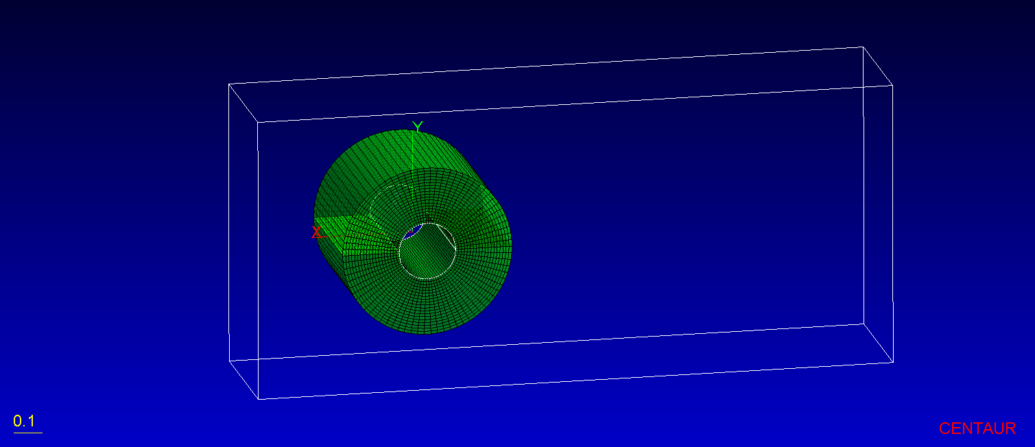
Cylinder Geometry with Block.

Use the FlowField>Setup… option or the corresponding toolbar icon to provide the mesh and solution files.

In the pop-up window, the Files tab is used to define the necessary mesh and solution files. First, set the Format to OpenFOAM and then provide the input files using the Browse buttons to navigate to the folder where the necessary tutorial files are stored:

Mesh: cylinder.hyb_OpenFOAM
Solution: folder named 50 (within the cylinder.hyb_OpenFOAM folder)
Mesh (CENTAUR fromat): cylinder.hyb

The Output file, named post file, is a special CENTAUR mesh including solution data that will be created after visualization is run. For this tutorial, keep the default file path and name.

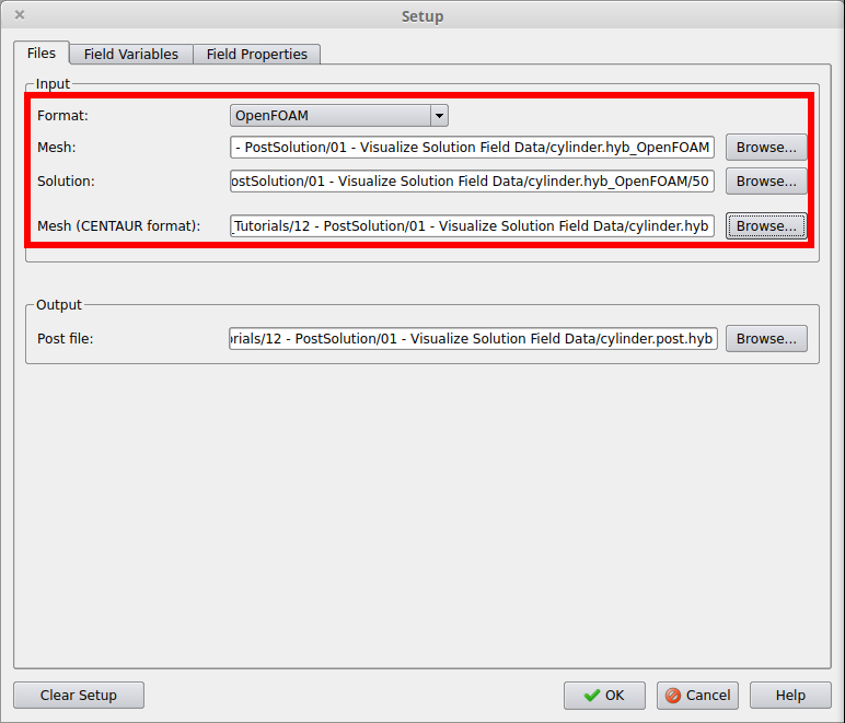
Files Tab in the Setup Window.

Step 2: Select Solver Variables for Visualization

Next, switch to the Field Variables tab of the Setup window to select which field variables will be visualized. The selected variables will also be written in the post file. Field variables are categorized as Solver variables and Custom variables. The former are retrieved from the provided solution file, whereas the latter are user-specified variables that are calculated within CENTAUR.

Enable the Solver variables option via the checkbox and click the Select… button to specify the subset of solver variables to be visualized.

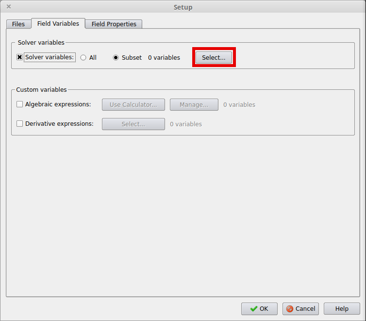
Define a Subset of Solver Variables to be Visualized.

In the Choose Solver Variables window, choose Ux, Uy, Uz and p and move them to the Selected Variables field using the > button. In this way, only the Ux, Uy, Uz and p variables will be available for visualization.

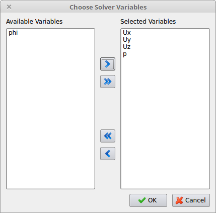
Choose Solver Variables Window.

Click OK to apply your selection. The number of the selected variables is reported in the Setup window. Next, click the OK button to confirm the Setup options and dismiss the window.

Step 3: Visualize Solution Data

Now that the setup is ready, the Run Visualization option is enabled in the FlowField menu. Clicking on it brings up an Output window with text regarding the running visualization process. After the process is finished, a popup window prompts for loading the created mesh/solution file, as well as for creating mesh cuts upon import.

Enable the Create meshcuts checkbox and click Yes in the popup window. In the Mesh Cut Setup window that appears, set up a Planar/Axis-aligned mesh cut at Z = 0.25, by selecting Direction Z and clicking the button Middle.

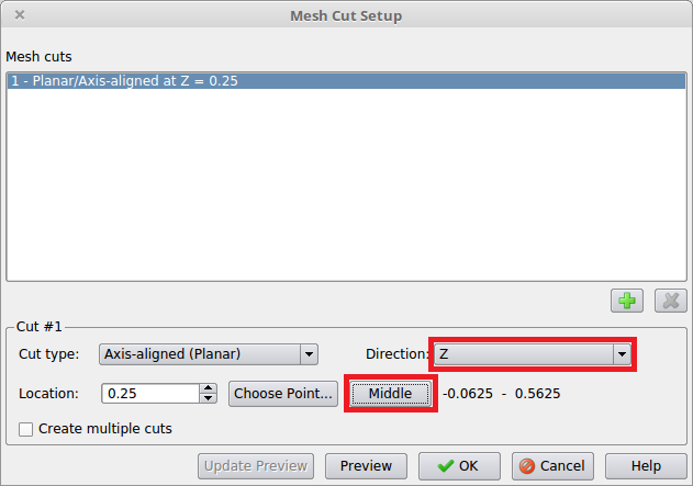
Create Cuts.

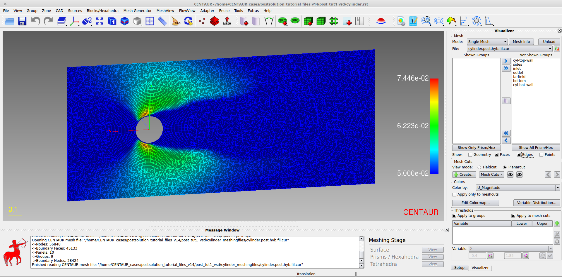
Upon clicking OK, the Visualizer sidebar is added to the left of the screen and the Ux variable appears in the display area. To see the values in the interior of the computational domain and specifically on the created meshcut, move all groups to the Not Shown Groups using the >> button and uncheck the Geometry checkbox.

Additionally, in the Colors block of the sidebar set the Color by option to U_Magnitude. That is the magnitude of the velocity, which was automatically calculated.

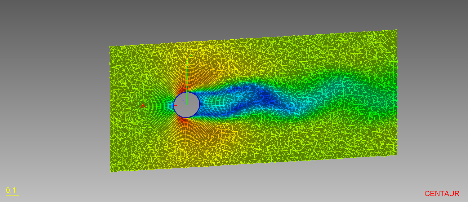
The screen should now look like the one in the following image:

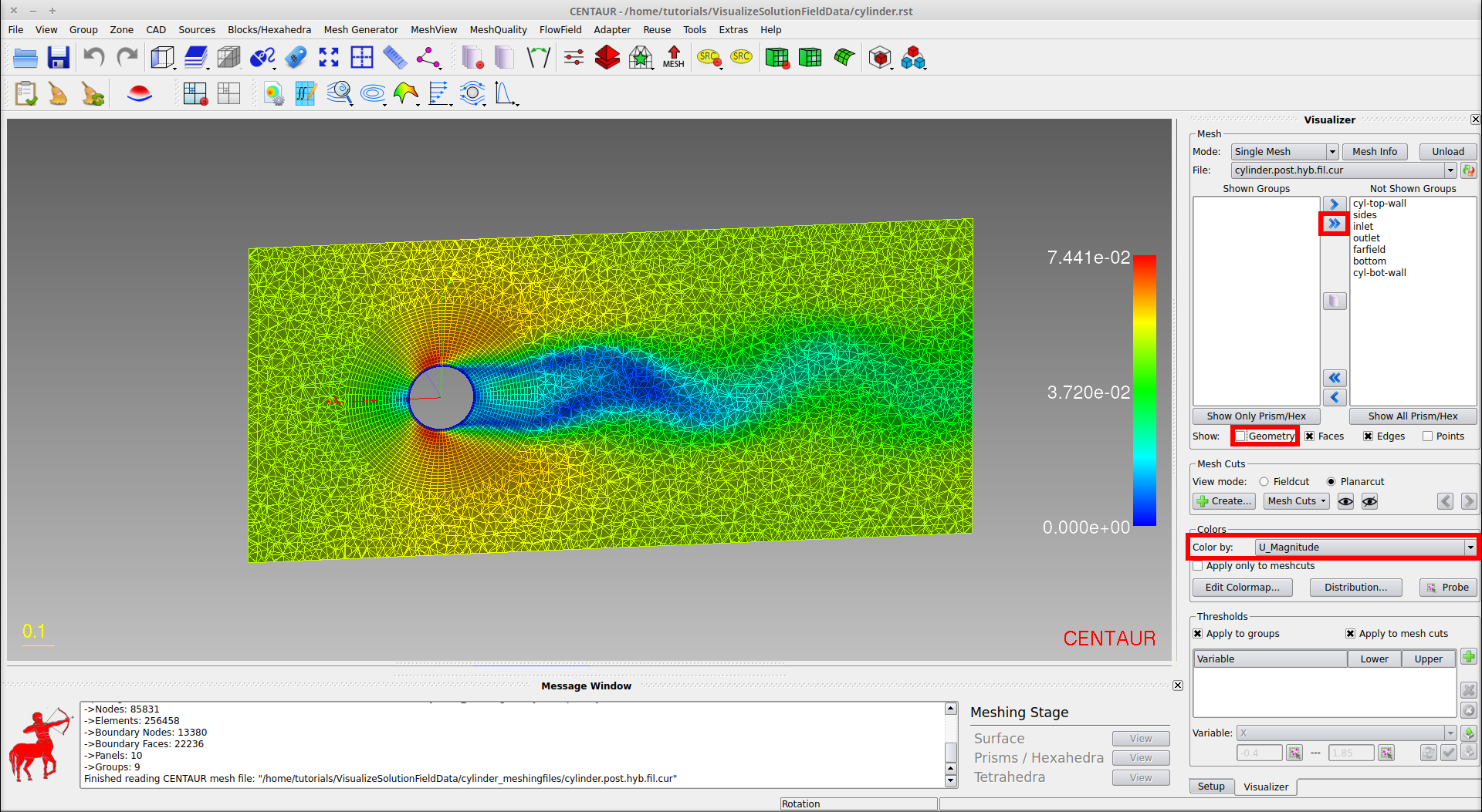
Mesh Cut Colored by Velocity Magnitude.

The Visualizer sidebar contains information regarding the selected variable. Click the Distribution… button (below the colorbar in the sidebar) to see a histogram with the distribution of U_Magnitude values:

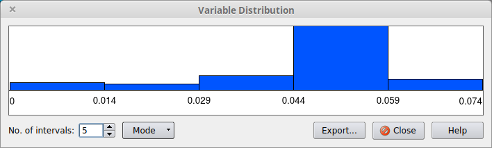
Histogram with Velocity Magnitude Values.

Clicking on the bins of the histogram will “isolate” in the graphics display area the portion of the mesh exhibiting the selected values. For example, by selecting the first two bins (hold the Ctrl button and click on each bin) the local mesh regions where the velocity magnitude values range from 0 to 2.98e-02 will be displayed, as shown below:

Local Mesh Regions Exhibiting the Specified Velocity Magnitude Values.

Click Close to dismiss the Variable Distribution window and then, click the Edit Colormap… button in the Visualizer sidebar. Set the minimum value of the field variable (Var. min parameter) to 0.05 in order to examine regions with flow accelerated to velocity higher than the inlet velocity.

Color Map Editor.

The result can be appreciated in the following image:

Manually Rescaled Velocity Magnitude Values.

Similarly, all the field variables stored in the post file can be inspected.

Step 4: Visualize Custom Field Variables

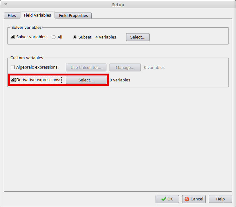
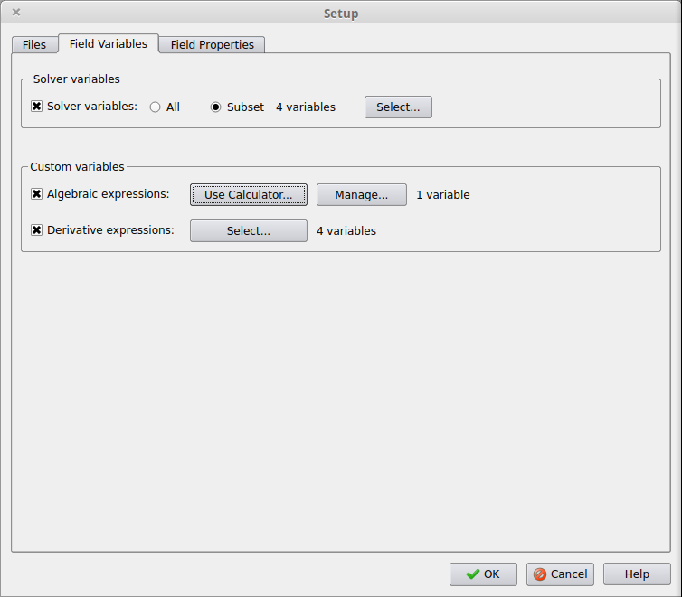
In this step, the Setup will be augmented for custom field variables to be visualized as well. Custom field variables can be:

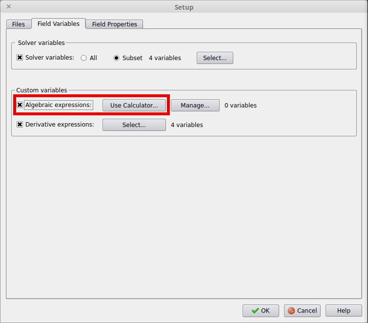
Algebraic expressions, which are constructed using algebraic operations on solver variables
Derivative expressions, which are derived from solver variables or algebraic expressions using differential operations

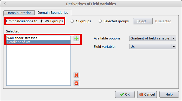
For the calculation of some derivative expressions (e.g. wall shear stress), it is necessary to map the solution variables founded in the provided solution file and define some properties of the flow field. This is done in the Solution tab of the Setup window.

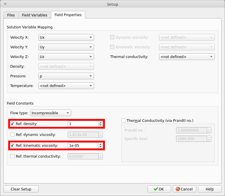
Re-open the Setup window either via the FlowField>Setup… option or via the toolbar icon , and switch to the Field Properties tab. Notice that the Solution Variables Mapping options are automatically filled in. In the Field Constants block of the window, retain the Flow Type as Incompressible and enable the Ref. density and Ref. kinematic viscosity parameters; set their values to 1.0 and 0.00001, respectively. These are the values that have been used by the solver.

Field Properties Tab in the Setup Window.

Next, switch to the Field Variables tab, enable the Derivative expressions option and click the corresponding Select… button, as shown below:

Select Derivative Expressions for Visualization.

This opens the Derivatives of Field Variables window. Two tabs exist, one for variables defined in the Domain Interior and another for variables defined only on the Domain Boundaries. In the Domain Interior tab, click the add button (+) to select the quantities to be calculated. The Gradient of Ux appears as the default selection. To change it, go to the Available options drop-down list and select Vorticity:

Select Vorticity.

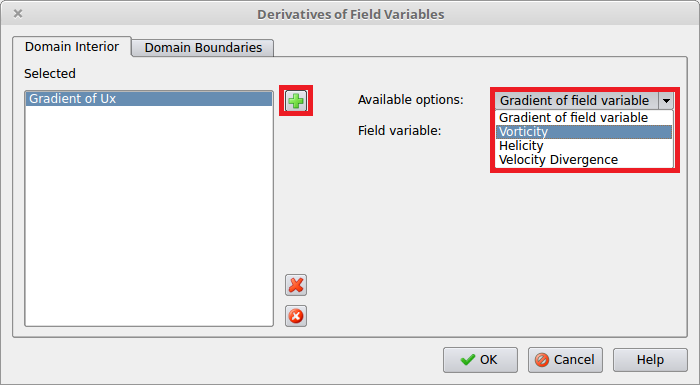
Similarly, add the gradient of pressure by hitting the add button (+) again, keeping the default option (Gradient of field variable), and selecting pressure (p) from the Field variable drop-down list.

Finally, switch to the Domain Boundaries tab and click the add button (+) to add the Wall shear stress from the drop-down list of the Available options. In the same way, click the add button (+) to keep the default Gradient of Ux, which already appears in the Selected list. Note that the current operation will calculate the gradient of the Ux velocity component, in direction normal to the boundary.

Select Wall Shear Stress and Gradient of Ux.

On the top of the window, set the Limit calculation option to Wall groups and click OK to dismiss the window. The Setup window is now updated with the number of selected Derivative expressions.

Additionally, an algebraic expression will be calculated and used for visualization. Specifically, the skin friction coefficient will be defined using the calculator. To do so, enable the Algebraic expressions option in the Setup window and click the Use Calculator… button:

Select Algebraic Expressions for Visualization.

In the Calculator popup window, set the Variable name to Cf. The Solution Variables drop-down list contains all solver variables stored in the solution files, as well as the Derived expressions that have been previously selected. Select the Wall_Shear_Stresses variable and type in the definition of the friction coefficient based on the magnitude of the inlet velocity, as it appears in the image that follows:

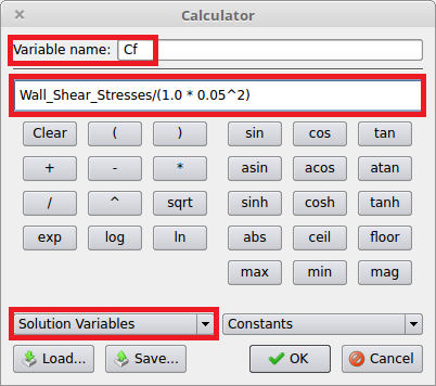
Formulate Algebraic Expression.

Click OK to dismiss the Calculator window. The Algebraic expressions field is updated with the number of defined expression. To inspect or modify the defined expression, click the Manage button.

The Field Variables tab of the setup window now looks as shown below:

Field Variables Tab in the Setup Window.

Click OK to dismiss the Setup window and proceed with the visualization of the selected field variables.

Step 5: Rerun Visualization

Use the FlowField>Run Visualization option to re-process the visualization data. Note that since the output filename was not changed in the Files tab of the Setup window, the existing post file will be overwritten. When the process is finished, click Yes in the popup window to load the new post file and the previously used mesh cuts.

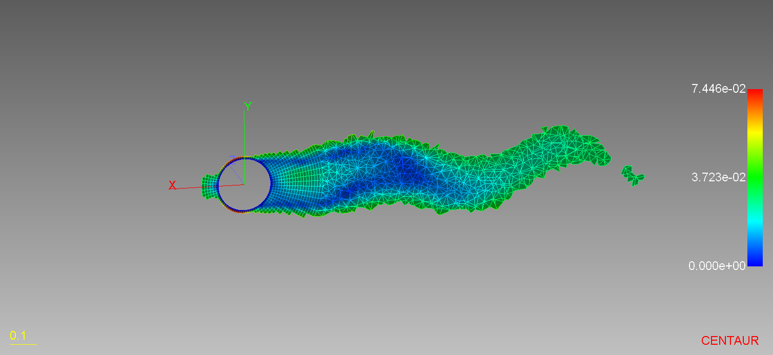
Set the Color by option to Vorticity_Magnitude, which was calculated along with the vorticity components, to plot the derived field quantity:

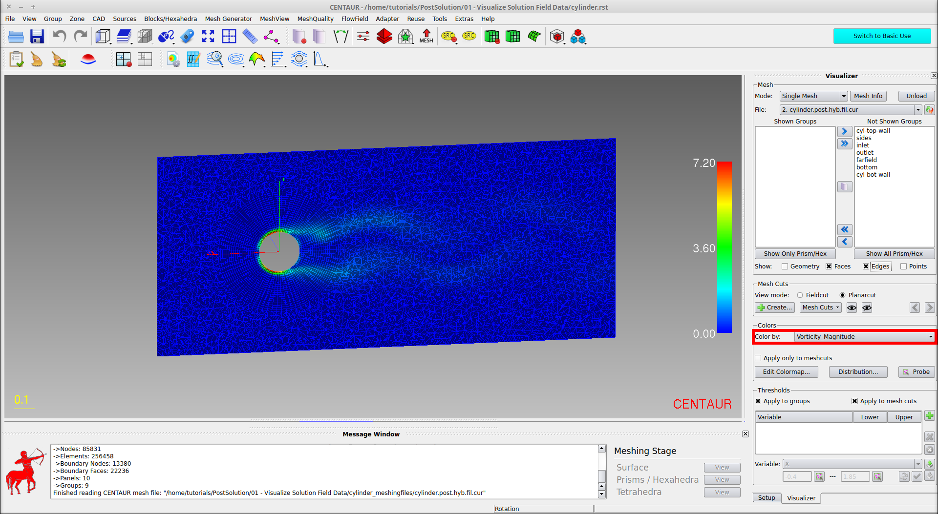
Mesh Cut Colored by Vorticity Magnitude.

The variable to be plotted next is the skin friction coefficient (Cf). Set the Color by option to Cf and the display shows the corresponding values on the planar cut. Recall that when constructed, Cf was defined only for Wall Boundaries. Therefore, click the Show All Prism/Hex button to move all the wall groups to the Shown Groups list and click the hide the meshcut using the corresponding button. In this way, the values of Cf can be visualized on the cylinder walls. The display appears in the following image:

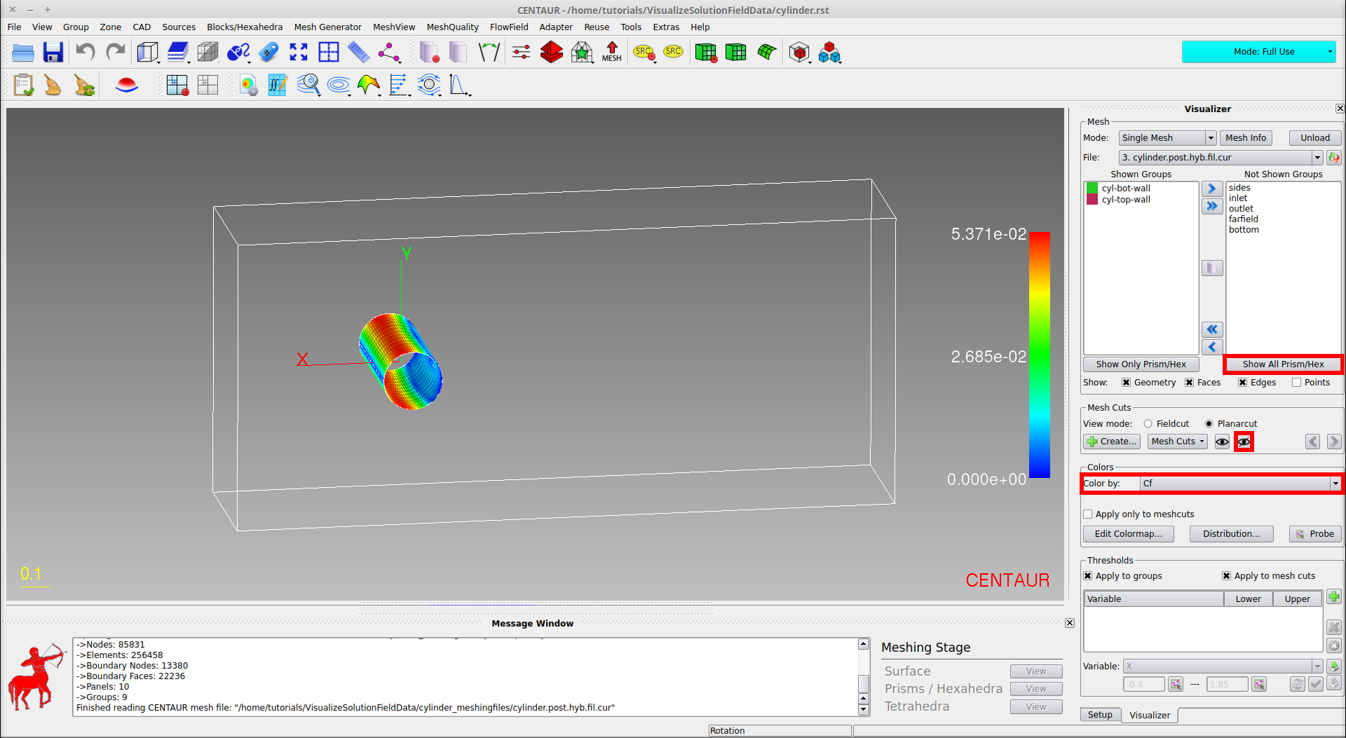
Surface Mesh Colored According to Skin Friction Coefficient.

More Information

For more information regarding the flow visualizer, as well as the other PostSolution tools that are available, please see the Solution Post-Process feature page.